Introduction

With Neural Radiance Fields (NeRFs), we can store a 3D scene as a continuous function. This idea was first introduced in the original NeRF publication [5]. Since then, the field experienced many advancements. Some of them even in the subsea domain. However, these advancements still have some limitations. This implementation adresses some of those limitations and provides a modular and documented implementation of a subsea specific NeRF that allows for easy modifications and experiments.

Approach

The fundamental principle underlying NeRFs is to represent a scene as a continuous function that maps a position, \(\mathbf{x} \in \mathbb{R}^{3}\), and a viewing direction, \(\boldsymbol{\theta} \in \mathbb{R}^{2}\), to a color \(\mathbf{c} \in \mathbb{R}^{3}\) and volume density \(\sigma\). We can approximate this continuous scene representation with a simple Multi Layer Perceptron (MLP). \(F_{\mathrm{\Theta}} : (\mathbf{x}, \boldsymbol{\theta}) \to (\mathbf{c},\sigma)\).

It is common to also use positional and directional encodings to improve the performance of NeRF approaches. Furthermore, there are various approaches in order to sample points in regions of a scene that are relevant to the final image. A detailed explanation of the exact implemented architecture is given in the Network architecture section.

Image formation model

The authors of [3] combine the fundamentals of NeRFs with the following underwater image formation model proposed in [1]:

\[I = \overbrace{\underbrace{J}_{\text{colour}} \cdot \underbrace{(e^{-\beta^D(\mathbf{v}_D)\cdot z})}_{\text{attenuation}}}^{\text{direct}} + \overbrace{\underbrace{B^\infty}_{\text{colour}} \cdot \underbrace{(1 - e^{-\beta^B(\mathbf{v}_B)\cdot z})}_{\text{attenuation}}}^{\text{backscatter}}\]

\(I\) …………… Image

\(J\) …………… Clear image (without any water effects like attenuation or backscatter)

\(B^\infty\) ……….. Backscatter water colour at depth infinity

\(\beta^D(\mathbf{v}_D)\) … Attenuation coefficient [1]

\(\beta^B(\mathbf{v}_B)\) … Backscatter coefficient [1]

\(z\) …………… Camera range

This image formation model allows the model to seperate between the clean scene and the water effects. This is very useful since it allows for filtering out of water effects from a scene. Some results where this was achieved are shown in the Results section.

Rendering equations

As NeRFs require a discrete and differentiable volumetric rendering equation, the authors of [3] propose the following formulation:

\[\hat{\boldsymbol{C}}(\mathbf{r}) = \sum_{i=1}^N \hat{\boldsymbol{C}}^{\text{obj}}_i(\mathbf{r}) + \sum_{i=1}^N \hat{\boldsymbol{C}}^{\text{med}}_i(\mathbf{r})\]

This equation features an object and a medium part contributing towards the final rendered pixel colour \(\hat{\boldsymbol{C}}(\mathbf{r})\). Those two components are given by:

\[\hat{\boldsymbol{C}}^{\text{obj}}_i(\mathbf{r}) = T^{\text{obj}}_i \cdot \exp (-\boldsymbol{\sigma}^{\text{attn}} t_i) \cdot \left(1 - \exp({-\sigma^{\text{obj}}_i \delta_i})\right) \cdot \mathbf{c}^{\text{obj}}_i\]

\[\hat{\boldsymbol{C}}^{\text{med}}_i(\mathbf{r}) = T^{\text{obj}}_i \cdot \exp (-\boldsymbol{\sigma}^{\text{bs}} t_i) \cdot \left(1 - \exp({-\boldsymbol{\sigma}^{\text{bs}} \delta_i})\right) \cdot \mathbf{c}^{\text{med}}\]

, with

\[T^{\text{obj}}_i = \exp\left(-\sum_{j=0}^{i-1}\sigma^{\text{obj}}_j\delta_j\right)\]

The above equations contain five parameters that are used to describe the underlying scene: object density \(\sigma^{\text{obj}}_i \in \mathbb{R}^{1}\), object colour \(\mathbf{c}^{\text{obj}}_i \in \mathbb{R}^{3}\), backscatter density \(\boldsymbol{\sigma}^{\text{bs}} \in \mathbb{R}^{3}\), attenuation density \(\boldsymbol{\sigma}^{\text{attn}} \in \mathbb{R}^{3}\), and medium colour \(\mathbf{c}^{\text{med}} \in \mathbb{R}^{3}\).

I use the network discussed below to compute those five parameters that parametrize the underlying scene.

Network architecture

The network implemented for this approach has the following architecture:

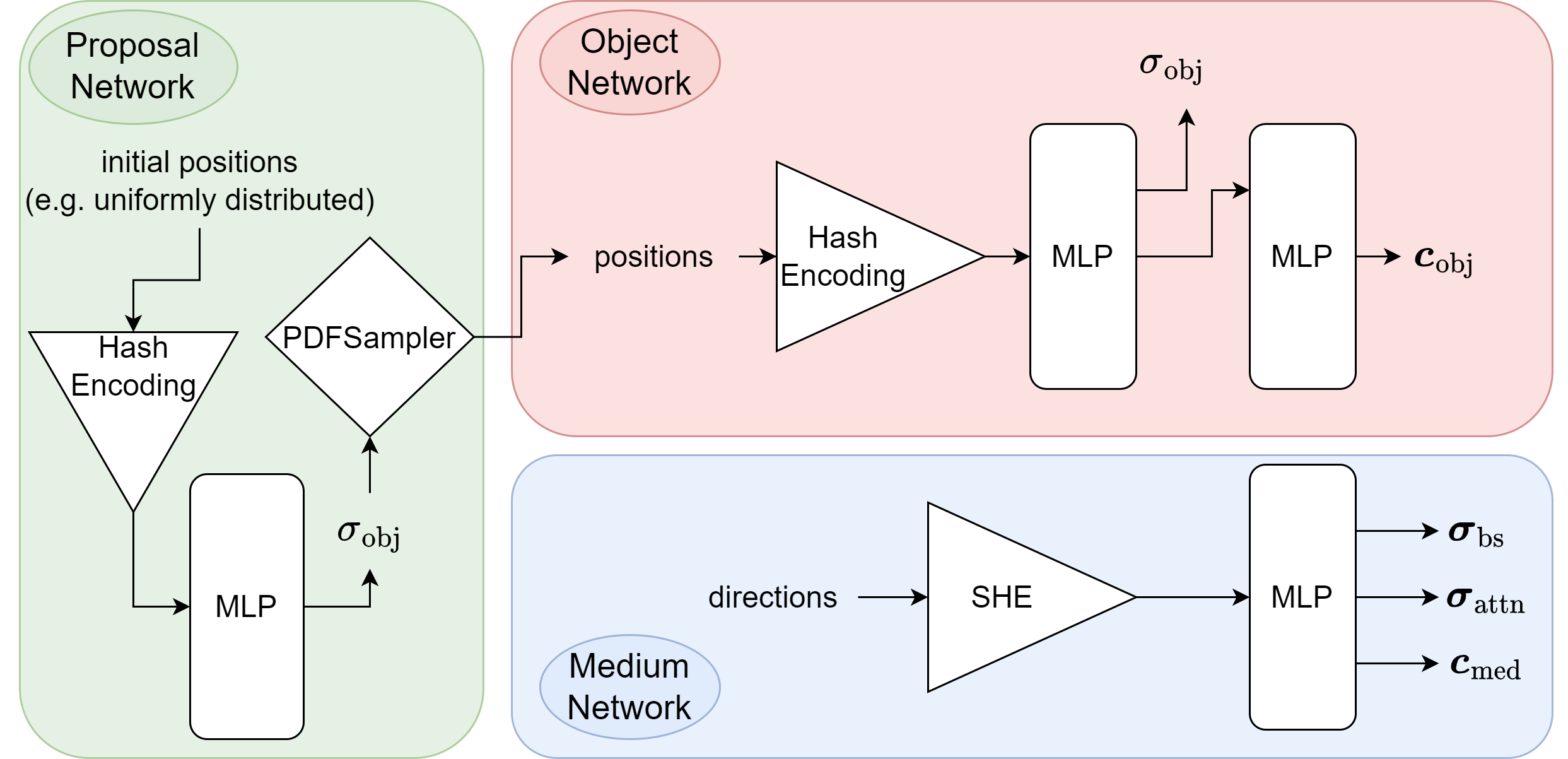
The object network computes \(\sigma^{\text{obj}}_i\) and \(\mathbf{c}^{\text{obj}}_i\), while the medium network computes \(\boldsymbol{\sigma}^{\text{bs}}\), \(\boldsymbol{\sigma}^{\text{attn}}\) and \(\mathbf{c}^{\text{med}}\).

The proposal network is used to sample point in regions of the scene that contribute most to the final image. This approach actually uses two proposal networks that are connected sequentially. More details on the concept of proposal samplers and how they are optimized during training can be found in [2].

For positional encoding, I use Hash Grid Encodings as proposed in [4] and for directional encoding I use Spherical Harmonics Encoding (SHE) introduced in [6].

The MLPs in the object and medium networks are implemented using tinycuda-nn for performance reasons.

Footnotes

[1] (1,2)

Those depend on range, object reflectance, spectrum of ambient light, the camera’s spectral response, and the physical scattering and beam attenuation coefficients of the water, all of which are wavelength-dependent.

References

[1]

Derya Akkaynak and Tali Treibitz. A revised underwater image formation model. In Proceedings of the IEEE Conference on Computer Vision and Pattern Recognition (CVPR). 6 2018.

[2]

Jonathan T. Barron, Ben Mildenhall, Dor Verbin, Pratul P. Srinivasan, and Peter Hedman. Mip-nerf 360: unbounded anti-aliased neural radiance fields. CVPR, 2022.

[3] (1,2)

Deborah Levy, Amit Peleg, Naama Pearl, Dan Rosenbaum, Derya Akkaynak, Simon Korman, and Tali Treibitz. Seathru-nerf: neural radiance fields in scattering media. 2023. arXiv:2304.07743.

[4]

Thomas Müller, Alex Evans, Christoph Schied, and Alexander Keller. Instant neural graphics primitives with a multiresolution hash encoding. ACM Trans. Graph., 41(4):102:1–102:15, July 2022. doi:10.1145/3528223.3530127.

[5]

Ben Mildenhall, Pratul P. Srinivasan, Matthew Tancik, Jonathan T. Barron, Ravi Ramamoorthi, and Ren Ng. Nerf: representing scenes as neural radiance fields for view synthesis. In ECCV. 2020.

[6]

Dor Verbin, Peter Hedman, Ben Mildenhall, Todd Zickler, Jonathan T. Barron, and Pratul P. Srinivasan. Ref-NeRF: structured view-dependent appearance for neural radiance fields. CVPR, 2022.